Analyzing Blog Performance Using R
When putting out content on the internet, it's interesting to see how everything performs, especially over time. While some topics might gain relevance, others may become less important. This is affected by broader trends in the industry, but also the nature of the content itself. Some blogs are dedicated to one specific topic, others vary their focus.
I'm writing these posts because they usually reflect what I'm doing at the time. In most cases, I'm trying to write down something I've learned to access it in the future when it becomes relevant again. Especially in phases where I have a lot of things going on at once, it helps to externalize all the knowledge that I don't need at all times.
In recent months, I learned the basics of Statistics, from the most basic things such as the arithmetic mean, median, and other measures of dispersion and central tendency, to probability theory and statistical inference with confidence intervals and statistical tests. And because we're in academia, there's a lot of (usually interesting) theory behind all of it.
Since I'm better at learning things I can apply in practice, I'm planning to periodically reflect and analyze the performance of my blog and other projects, using some of the things I learned. Over time, this will help me to retain what I learned in the module while also giving everyone who's interested some insights.
This post starts the exploration of this blog's performance in the last 365 days, with data provided by the Google Search Console. I don't have any analytics set up for this blog, which I might have to change if I need more than impressions, clicks and search keywords in the future.
I still think the search data is a relatively accurate measure of how this site performs, as most people and software engineers are using Google. I don't think users of other search engines search for much different content, making the data I'm able to export relatively realistic as a sample.
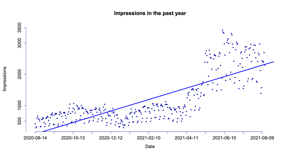
These first steps are quite important for determining what our goal is when applying statistical measures. In my case, I want to see the historical performance in terms of impressions and clicks, and draw a regression line, which acts as a forecast for future performance based on the data we have at hand.
Due to the nature of linear regression, if I wanted to use this for real decisions, I'd have to evaluate how well it fits in terms of errors, for example by decomposing the dispersion into explained parts based on our data, and the remaining values (residuals).
Exploring and Preparing our Data
Let's start by exploring our available data. For this post, we'll use the historical data that includes the date of measurement, clicks, impressions, CTR (clicks / impressions), and position sorted by date descending.
Date,Clicks,Impressions,CTR,Position
2021-08-13,65,2296,2.83%,29.97
2021-08-12,105,2695,3.9%,26.65
2021-08-11,97,2385,4.07%,26.59
To revert our variables, we'll use rev. We'll also convert our dates into the days from 1 to 365, as we can't use the dates in text representation. For this, we assume that there are no gaps (i.e. that we have a record for each of the 365 days).
# Read our file (365 records with 5 variables)
data <- read.csv("./blog/data.csv", header = TRUE)

# Retrieve variables we'll use, reverse order
impressions <- rev(data$Impressionen)
clicks <- rev(data$Klicks)

# Convert dates to days (1 to 365)
dates <- rev(data$Datum)
rowNum <- seq(from = 1, to = length(dates), by = 1)
Once our variables are prepared, we can create our regression line. For this, we simply use the lm function to create linear model, adding in the formula y=x as y~x. In our case, entering date results in impressions or clicks for the respective plot.
# Create regression line
regressionImpressions <- lm(impressions~rowNum)
regressionClicks <- lm(clicks~rowNum)
Once we have our regression lines ready to use, let's plot them!
Plotting our Data
Before we get started, we add some margin so we get enough space for axes and labels.
We'll use the default plot function, so we need to insert x and y value vectors. These have to be numeric, so we'll pass the row numbers (sequence from 1 to 365) as x and our impressions as y.
Then, we'll configure what our data points should look like. In our case, I've chosen small black dots. The scaling factor cex determines the size, 1 is 100%.
As we will cover all axes and labels ourselves, we'll set axes and ann (labels, title) to false.
par(
  # Margin to (bottom,left,top,right)
  mar = c(6,6,6,6) + 0.1
)

# Create first scatter plot for impressions
plot(
  x = rowNum, y = impressions,
  # Display black dot scaled to 75% (smaller)
  pch = 16, col = "#0100a4", cex = 0.75,
  # Do not draw axes or title, we'll do it ourselves
  axes = FALSE, ann = FALSE
)
At the moment, we can only see the data points. Let's continue to add our regression line, followed by the axes and axis titles.
# Add regression line into plot
abline(regressionImpressions, col="#0200ff", lwd=3)

# Break down dates for labels, create label every 30 days
reducedIdx <- seq(1, length(dates), 30)
reducedDates <- as.Date(dates[reducedIdx])

# Add labelled x axis
axis(1, at = reducedIdx, labels = reducedDates, col = "#0100a4",  cex.axis = 1.25)

# Add labelled y axis
axis(2, at = c(100,500,1000,2000,3000,3500), col = "#0100a4", cex.axis = 1.25)

title(
  ylab = "Impressions",
  # Distance to plot edge
  line = 4.5,
  cex.lab = 1.25,
)

title(
  xlab = "Date",
  # Distance to plot edge
  line = 3,
  cex.lab = 1.25
)

title(main = "Impressions in the past year", cex.main = 1.5)
And that's all we need. If we preview our plot, we should see the following.
We can repeat the same for clicks to end up with the following plot
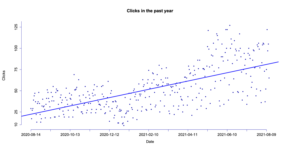
There's a lot more fluctuation in the impressions, which is natural. Clicks represent real interactions and should be the data set we're focusing on primarily. Due to the strong volatility, the regression line is not as suitable for impressions as it is for clicks.
Forecasting
Now that we roughly know our trends, let's try to peek into the future a bit. With our regression line, we have a classic linear function with an intercept and slope. While we can check out the forecasted value for every known day, we can also extend it into the future.
Based on how linear regression works, we can only forecast patterns based on the existing data we used to create the regression line. This means that we cannot forecast unexpected trend changes. It's only a continuation of what we already know, and whether that is realistic or not, we'll only know in the future.
# Extract intercept and slope
intercept <- regressionClicks$coefficients[1]
slope <- regressionClicks$coefficients[2]

# Create a linear function from it
forecast <- function (days) {
	as.numeric(intercept) +as.numeric(slope) * days
}

# Forecast clicks after a year (i.e. 2021-08-14)
forecast(365 * 1) # 81.64316

# Forecast two years into the future (i.e. 2022-08-14)
forecast(365 * 2) # 141.1363
As you can see, our forecast tells us that we'd be at 141 clicks in August of 2022. Let's see if we can hit this milestone.
I hope you enjoyed this first exploration of this blog's performance. There's much more to cover, in future issues we'll see if we can detect some patterns, for example, if readers are more active on specific days!